In traditional art, we paint with a physical thing: acrylic, oil, watercolor. In digital art, we paint with numbers and light. In this post, we examine the process of representing the complexity of human vision with simple numbers. This journey will take us from the emission of light by screens, to the stimulation of the biological eye, and ultimately to the perception of a color in the brain. Along the way, we will learn what many color acronyms mean: RGB, LMS, LAB, Oklab, sRGB, ACES, Rec. 2020, XYZ, HSV, and HSL.
Emission from the Screen: RGB
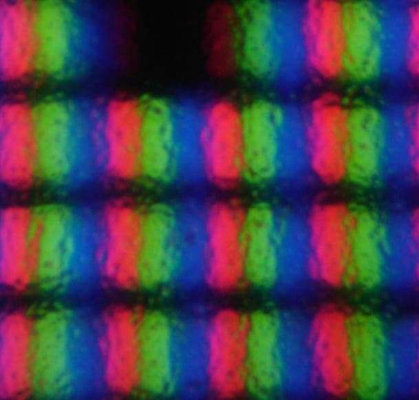
Our journey begins with a screen emitting light. Our screens are very small red, green, and blue elements side by side. Under magnification, like in the image of LCD TN subpixels, the individual red, green, and blue elements are visible; further away, they blend together to produce the wonderful spectrum of colors we see.

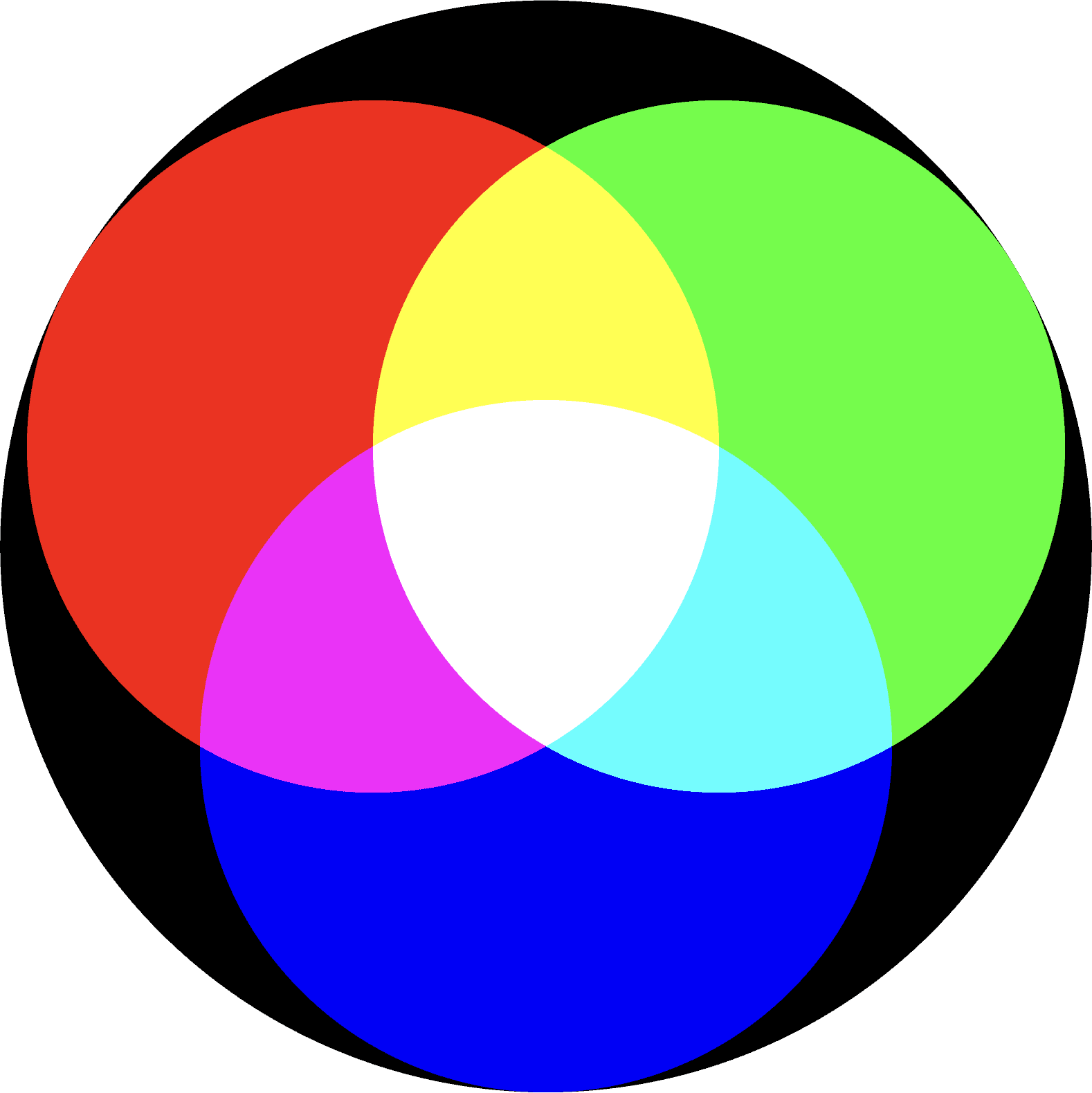
The most common representation of colors in digital art is RGB. The R stands for the red element, the G for the green element, and B for the blue element. When we use an RGB color, what we are really doing is controlling how much light the red, green, and blue elements on a display produce. When we do this, we blend the light of the three colors: all on to make white, just the blue one on to make blue, red and blue on together to make magenta, and so on.
You may ask: Wait, red and blue make magenta? When I mix red and blue paint I get purple.
Mixing colors on a computer display is different from mixing paint, similar, yet crucially different. Paint absorbs and reflects light; displays emit light directly. If we turn on red and blue lightbulbs side by side they meld to a lighter magenta color. If we mix red and blue paint they produce a darker purple color. Both colors are similar in hue but different in brightness.
From the Screen to Your Eye: LMS
The screen is emitting red, green, and blue light into your eye. Now, biology takes over as cells inside your eye are stimulated by the light. In this section, we talk briefly about how this works and the niche, but cornerstone, color format LMS (long, medium, short).
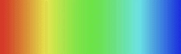
First, we need to get a sprinkle of physics out of the way. Light is a form of electromagnetic radiation. Electromagnetic radiation comes in a spectrum of wavelengths. Visible light is a sliver of that spectrum. We have UV (ultraviolet) and IR (infrared) adjacent to the visible spectrum. Radio, gamma waves, and X-rays are also part of the same physics phenomenon as visible light. Within the visible spectrum, we see different wavelengths as different colors.
 Infrared
As you may recall from high school biology, we have two classes of photoreceptor cells: rods and cones. Rods are mostly for low-light vision, so for our color discussion we only concern ourselves with cones. Scientists have prodded human vision and discovered that we have three groupings of cone cells, cells that are stimulated by long, medium, and short wavelengths of light. The sensitivity of the three cone classes to different wavelengths of light is the biological impetus for our vision.
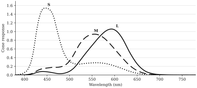
We can now define the acronym LMS. It is a numerical representation of how sensitive of our long, medium, and short cone cells are to a given wavelength of light, or more simply, a numerical representation of how our eyes see color biologically. For a selection of colors from across the visible spectrum, their LMS values are below.
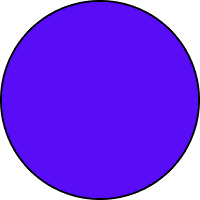 450 nmL = 0.074, M = 0.161, S = 1.534
 496 nmL = 0.066, M = 0.277, S = 0.354
 542 nmL = 0.580, M = 0.908, S = 0.274
 588 nmL = 1.050, M = 0.738, S = 0.245
 634 nmL = 0.512, M = 0.215, S = 0.083
 680 nmL = 0.042, M = 0.016, S = 0.006
From Your Eyes to Your Brain: LAB
Light is now stimulating cone cells inside the eye and a signal is pulsing to the brain. Our journey takes us to the mysterious realm of the mind and the color representation that describes it, LAB. LAB defines a color as a lightness L plus two color components A and B.
To understand A and B, let us first imagine some mixes of color. Let's think about mixing reds, greens, blues, and yellows.
If you tried to define a reddish blue, you would describe a purple color.
+=A reddish yellow would give you an orange color.
+=Greenish blue produces a teal color.
+=And a greenish yellow will give you a lime color.
+=Now, try to visualize a reddish green or a bluish yellow. As hard as you may try, you cannot visualize these mixtures. There are no greenish-red or bluish-yellow we can think of.
These opposing pairs of colors are fundamental to the theory for how we perceive color, the opponent color theory. According to the opponent color theory, we perceive color in terms of light and dark, red and green and blue and yellow. These opponent colors are how we get from LMS to LAB, how we get from our biology into our mind. We now have all we need to define the LAB components.
L is for lightness and it is the first component of a LAB color. To get the lightness of a color from LMS we take the long wavelengths plus the medium wavelengths; the short wavelength receptors do not contribute to lightness.
A is the next component of LAB. It defines the red and green opponent colors. Positive values push us toward red and negative toward green. To get the red/green proportion, or A component, we take the long wavelengths and subtract the medium wavelengths.
B is the final component of LAB. It defines the blue and yellow opponent colors. Positive B push us toward yellow and negative B pushing us toward blue. To get the blue/yellow proportion, or B component, we take the long and medium wavelengths and subtract the short wavelengths.
To dive into the math, you can look at the exact formula for a conversion from LMS to Oklab (Oklab is one type of LAB color space) in From LMS to OkLab.
Yellow−A
Green
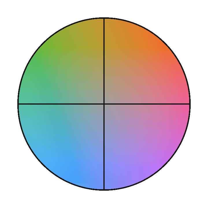 +A
+ARed−B
Blue
RGB vs LAB, Physical vs Perceptual
In digital art, a key distinction when representing a color with numbers is between physical and perceptual. Physical, such as RGB defines a color based on the physical properties of the display. A perceptual color, such as LAB, defines a color based on how we see it in our mind. While we can convert between physical and perceptual with formulas, defining which type of color we use controls how natural many effects look.


The choice of color representation controls how an edit behaves. RGB is useful when an operation models physical light, while perceptual spaces such as LAB are useful when an operation should follow human perception. We use that distinction throughout BrushCue's color adjustments, such as exposure, which scales linear RGB, and tinting, which shifts the Oklab A and B components.
sRGB, ACES, Rec. 2020 and Color Spaces
RGB, as we have seen, defines colors with respect to the physical property of a display. The trouble with this is that not all displays are the same. Furthermore, not all cameras are the same. The question then becomes, how do we make sure the color on your monitor looks the same as the one on someone else's monitor? The answer to this question is color spaces. Color spaces define what we mean when we say the R, G, and B are certain values. There are many color spaces that are commonly used depending on context: sRGB for web, ACES for professional filmmaking, Rec. 2020 for HDR video for example.
To convert between color spaces we need some agreed upon intermediate format that each conversion can go through. For that, the XYZ color space is the industry standard. We will take a closer look at color spaces in a future post. But, for now, suffice to say that color spaces are required to give meaning to RGB numbers.
What About HSV and HSL?
In your travels, you have probably seen HSV (and/or closely related, HSL), and you are unlikely to have seen LAB directly and you may therefore be wondering why we do not use HSV as our perceptual color. Here, I want to touch upon what HSV and HSL are and why they are not actually perceptual color formats.
Let's start by understanding how HSV is created. It is created by a simple mathematical transformation from RGB. To calculate the value or V component, we take the maximum of the R, G, and B channels. The saturation or S component is the difference between the max R, G, and B and the min R, G, and B divided by the max. And then the hue or H component points in the direction of the strongest of the R, G, and B channels. For the discussion here, it isn't too important. But, what you will see is that everything is based on R, G, and B. What we've learned in this post is that RGB defines how colors that are emitted and not colors that we perceive. Therefore, HSV (and HSL which is similarly defined) are related closely to RGB and not perceptual. Because of this, you will get into trouble when trying to do perceptual operations on HSV colors as opposed to LAB or other perceptual color formats.
 Saturation
 Value
Value